Technical Challenge
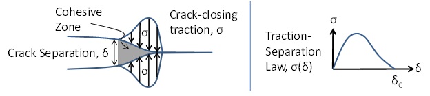
Cohesive zone modeling (CZM) is a powerful tool for predicting delamination in adhesively bonded structures and is widely implemented in commercial finite element codes. In the CZM approach (Figure 1), fracture is assumed to occur by progressive separation of the crack surfaces ahead of the crack tip. The crack grows when the crack separation reaches a critical value, δC. The key input into any cohesive zone model is the traction-separation law, σ(δ). The successful use of cohesive zone modeling relies upon this traction-separation law to represent accurately the fracture of the material or interface being modeled. The traction-separation law therefore must be calibrated experimentally.
Veryst Solution
We use our expertise in experimental and computational fracture mechanics to calibrate traction-separation laws for direct implementation into finite element models of adhesively bonded structures.
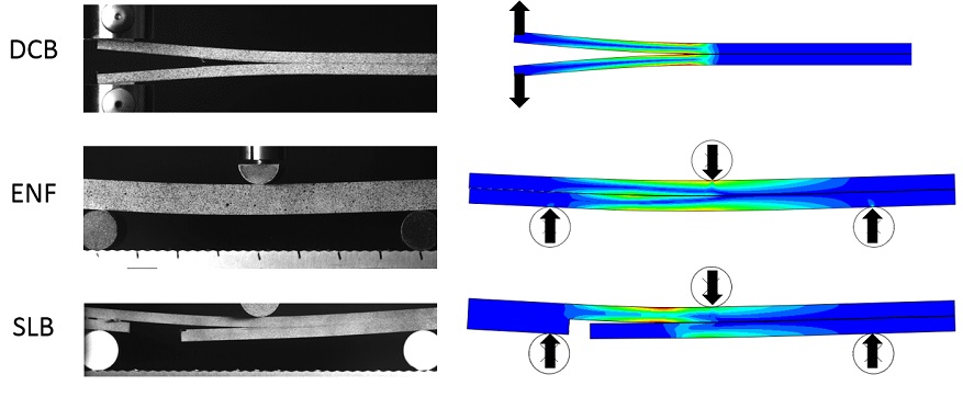
This is done by conducting an appropriate set of fracture mechanics based experiments. Test specimens that we commonly use include the double cantilever beam, end notch flexure, and four-point bend geometries (Figure 2). Other experiments may be employed depending upon the nature of the interface being tested. We present two examples below.
Example 1: Mode II Traction-Separation Law for a Brittle Adhesive
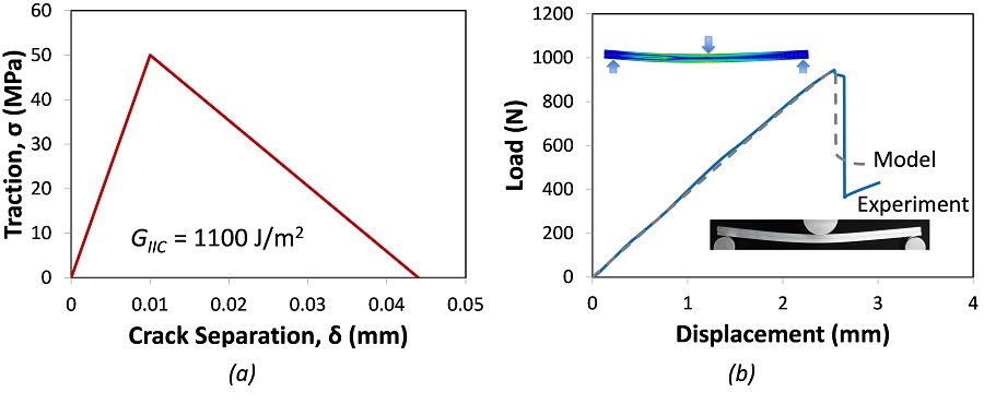
We calibrated a Mode II traction-separation law for a brittle epoxy using the end notch flexure (ENF) specimen. We simulated the test and iteratively found a bilinear tractions-separation law (Figure 3a) that accurately reproduced the experimentally measured ENF test load-displacement response (Figure 3b).
For brittle adhesives and interfaces, simple bilinear models are typically sufficient and computationally easy to implement. A similar procedure can be followed to model Mode I and Mixed Mode fracture.
Example 2: Mode I Traction-Separation Law for a Flexible Adhesive
When the deformation in the adhesive is large, the shape of the traction-separation law becomes important and can be calculated from direct measurement of the J-integral and the crack separation, δ, as the traction-separation law, σ(δ), is equal to the derivative of the J-integral with respect to δ:
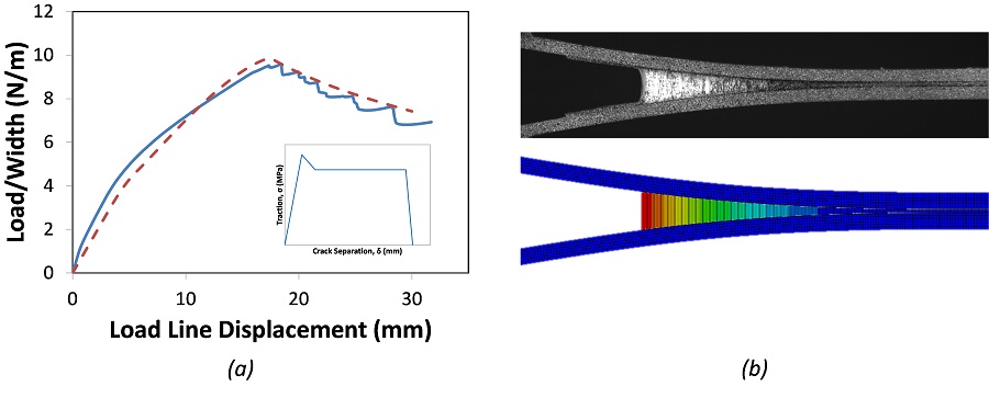
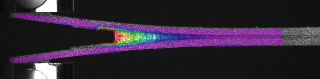
Experimentally, the crack separation is measured by the use of digital image correlation (Figure 4). The J-integral is calculated from the measured load and rotations of the bonded beams.
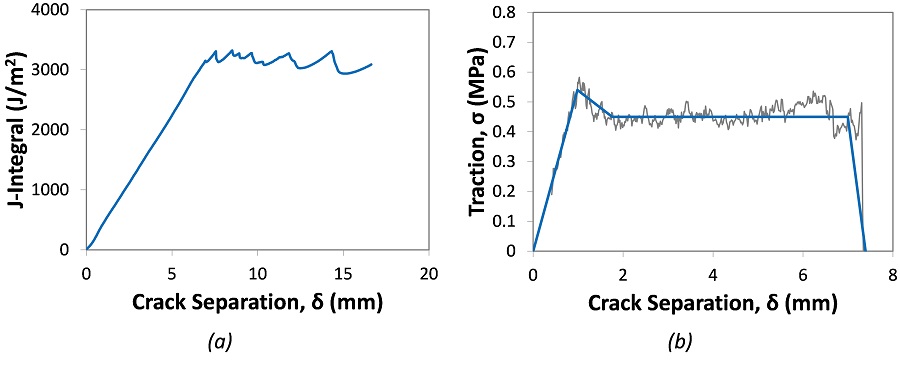
We tested the Mode I fracture of a flexible adhesive using the double cantilever beam geometry. Figure 5a shows the measured value of the J-integral with respect to crack separation, δ. The steady state fracture energy of the adhesive tested was about 3300 J/m2.
We compute the traction-separation law by taking the derivative of the J-integral with respect to δ as shown in Figure 5b. For the adhesive tested, fracture is characterized by a peak stress of 0.55 MPa, a large plateau at 0.45 MPa, and abrupt rupture of the adhesive at an elongation of about 7 mm. The solid blue line is a piecewise linear fit to the experimental data that can be used as input into a finite element model.
We compared the simulated and experimentally measured force-displacement curves of the DCB test to verify correct extraction and implementation of the model (Figure 6a).
Figure 6b compares a photograph of the specimen deformation at the onset of crack growth with the model prediction.